Autoencoders

High dimensional data is usually very structured, and this structure allows us to map the data to a smaller dimensional space without losing much information.  For example, if this post is encoded with ASCII, it lives in a \((256)^{\text{length post}}\) point space.  But since I’m writing in English, the sequence of characters “Life is a tale told by an idiot, full of sound and fury, signifying nothing” is far more likely than the sequence “fjkla;8#knxHJD38lkdf dfjkal.”  Thus my post really lives in a very low-dimensional “English subspace” of the full \((256)^{\text{length post}}\) point space.  The same principle applies to lots of other data.  For example, strictly speaking a 10 megapixel image is described by about 30 million numbers (about 10 million RGB triples), but since people take pictures of predictable things such as cats, dogs, faces, rocks, etc., you can describe the picture using much fewer than 30 million numbers.  Dimensionality reduction is used for image compression, audio compression, and video compression.  In learning algorithms, we have high dimensional feature vectors (e.g., the features could be the RGB values in an image), but the algorithms behave better if we first map the features to a low-dimensional space.

The problem is to map \(N\) dimensional data to a \(d\) dimensional code, and the goal is to learn an encoder \(f : \mathbb{R}^N \to \mathbb{R}^d\) and a decoder \(g : \mathbb{R}^d \to \mathbb{R}^N\) such that \(g(f(x)) \approx x\).  PCA (principal component analysis) is historically the most popular method of dimensionality reduction.  In PCA, both the encoder and decoder are linear maps and geometrically it’s finding a \(d\) dimensional hyperplane that the \(N\) dimensional data hovers around.  A more modern approach uses autoencoders.

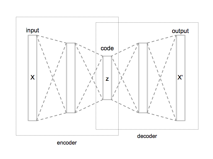
An autoencoder is a feed-forward neural network that we train so that the \(N\) dimensional output layer reconstructs the \(N\)-dimensional input layer.  Internally there is a hidden “code” layer with \(d\) nodes.  The encoder is the “bottom” part of the network mapping the \(N\) dimensional input layer to the \(d\) dimensional code layer, and the decoder is the “top” part of the network mapping the \(d\) dimensional code layer to the \(N\) dimensional output layer.  In training the autoencoder, we minimize

\[L(x, g(f(x))),\]

where the loss \(L\) tries to force the reconstruction \(g(f(x))\) to be close the input \(x\).  To prevent the autoencoder from learning the identity, we impose a structural constraint in the network by making \(d \ll N\), or we add regularization to the loss function and try to minimize

\[L(x, g(f(x))) + \Omega(h),\]

where \(h = f(x)\) is the hidden code layer, and \(\Omega\) imposes some structure on \(h\), e.g., sparsity.

Written on April 13th, 2018 by Scott Roy