Optimization and duality

Introduction

Consider the optimization problem

\[\begin{aligned} \inf_{x \in E} &\quad f(x) \\ \text{subject to} &\quad g(x) \leq 0, \end{aligned}\]

where the function \(g: \mathbb{R}^n \to \mathbb{R^p}\) defines \(p\) constraints. Constraints can also be built into the set \(E \subseteq \mathbb{R}^n\).

The Lagrangian

The Lagrangian is defined as

\[L(x, \lambda) = f(x) + \lambda^T g(x) = f(x) + \sum_{i=1}^p \lambda_i g_i(x).\]

In the Lagrangian, the “hard” constraints \(g_i(x) \leq 0, \ 1 \leq i \leq p,\) in the optimization problem are replaced with “soft” penalties that can be violated, but for a cost; cost \(\lambda_i\) is incurred per unit violation of the \(i\)th constraint (and credit given per unit “under budget”). A natural question is if there are “prices” \(\lambda\) for which

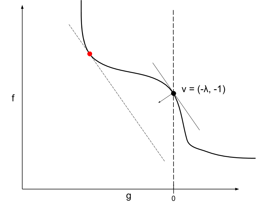
\[\Pi(\lambda) := \inf_{x \in E} L(x, \lambda) = \inf_{x \in E} f(x) + \lambda^T g(x)\]

has the same solution set as the original problem? This is not always the case, as the figure below illustrates. In the figure, the curve \(v(t) = \inf \{ f(x) : g(x) \leq t, x \in E \}\) is plotted, which we assume is the boundary of the region \(A = \{ (g(x), f(x)) : x \in E \}\). The problem that defines \(\Pi(\lambda)\) can be viewed as maximization of the linear functional \((g, f) \mapsto (-\lambda, -1)^T (g,f)\) over \(A\). The original problem corresponds to the point \((0, v(0))\), which cannot be obtained by maximizing a linear functional (note that the functional corresponding to the tangent at \((0, v(0))\) is maximized at the red dot).

Primal and dual problems

The connection between the original (primal) optimization problem and the Lagrangian is given by

\[p^* = \inf_{x \in E} \sup_{\lambda \in \mathbb{R}^n_+} L(x, \lambda),\]

where \(p^*\) is the primal optimal value. This is easy to see by noting that

\[P(x) := \sup_{\lambda \in \mathbb{R}^p_+} L(x, \lambda) = \left\{ \begin{matrix} f(x) &\quad \text{if } g(x) \leq 0 \\ \infty &\quad \text{otherwise} \end{matrix} \right. .\]

It is natural to consider the dual problem in which the order of the inf and sup are reversed:

\[d^* := \sup_{\lambda \in \mathbb{R}^p_+} \inf_{x \in E} L(x, \lambda).\]

The function \(\Pi(\lambda) = \inf_{x \in E} L(x, \lambda)\) is called the Lagrangian dual function.

The minimax inequality implies weak duality

\[d^* = \sup_{\lambda \in \mathbb{R}^p_+} \Pi(\lambda) = \sup_{\lambda \in \mathbb{R}^p_+} \inf_{x \in E} L(x, \lambda) \leq \inf_{x \in E} \sup_{\lambda \in \mathbb{R}^n_+} L(x, \lambda) = \inf_{x \in E} P(x) = p^*.\]

The minimax inequality and saddle points

The minimax inequality is

\[\sup_{y \in Y} \inf_{x \in X} f(x, y) \leq \inf_{x \in X} \sup_{y \in Y} f(x, y)\]

and holds for any function \(f\) and any sets \(X\) and \(Y\). To derive the inequality, start with

\[f(x, y) \leq \sup_{y \in Y} f(x,y),\]

then take an infimum on both sides

\[\inf_{x \in X} f(x, y) \leq \inf_{x \in X} \sup_{y \in Y} f(x,y),\]

and finish with a supremum over the left side

\[\sup_{y \in Y} \inf_{x \in X} f(x, y) \leq \inf_{x \in X} \sup_{y \in Y} f(x,y).\]

To illustrate the inequality in a simple setting, consider the discrete function \(f(i,j)\) whose values are enumerated in in the matrix below (\(f(1,1) = 1\), \(f(1,2) = 2\), \(f(2,1) = 3\), and \(f(2,2)=1\)).

\[\begin{matrix} \begin{bmatrix} 1 & 2 \\ 3 & 1 \end{bmatrix} & \begin{matrix} \color{green}{2} \\ \color{green}{3} \end{matrix} \\ \begin{matrix} \color{red}{1} & \color{red}{1} \end{matrix} & \end{matrix}\]

The minimax inequality says that the largest column min (1) is no more than the smallest row max (2). (The column mins are shown in red below the matrix, and the row maxes are shown in green to the right of the matrix.) This simple example shows that equality does not always hold.

Equality and saddle points

Equality holding in the minimax inequality is closely related to the existence of saddle points of \(f\). A saddle point \((\bar{x}, \bar{y})\) satifies

\[f(\bar{x}, y) \leq f(\bar{x}, \bar{y}) \leq f(x, \bar{y})\]

for all \(x \in X\) and \(y \in Y\). A saddle point implies equality holds in minimax:

\[\begin{aligned} \sup_{y \in Y} \inf_{x \in X} f(x,y) &\geq \inf_{x \in X} f(x, \bar{y}) \\ &\geq f(\bar{x}, \bar{y}) \\ &\geq \sup_{y \in Y} f(\bar{x}, y) \\ &\geq \inf_{x \in X} \sup_{y \in Y} f(x, y). \end{aligned}\]

In the discrete setting, a saddle point is an entry that is the largest in its row and the smallest in its column. For example, 2 is a saddle point in the matrix below because it is the biggest value in its row and the smallest value in its column (and minimax equality holds).

\[\begin{matrix} \begin{bmatrix} 1 & 2 \\ 3 & 4 \end{bmatrix} & \begin{matrix} \color{green}{2} \\ \color{green}{4} \end{matrix} \\ \begin{matrix} \color{red}{1} & \color{red}{2} \end{matrix} & \end{matrix}\]

Since a saddle point implies equality in minimax, it is natural to wonder the converse: if equality holds, does \(f\) have a saddle point? This is true as long as the optimal values are attained. Suppose \(\bar{x} \in X\) is optimal in that

\[\sup_{y \in Y} f(\bar{x}, y) = \inf_{x \in X} \sup_{y \in Y} f(x, y).\]

and \(\bar{y} \in Y\) is optimal in that

\[\inf_{x \in X} f(x, \bar{y}) = \sup_{y \in Y} \inf_{x \in X} f(x, y),\]

and equality holds in minimax. Then we have

\[\begin{aligned} \sup_{y \in Y} \inf_{x \in X} f(x,y) &= \inf_{x \in X} f(x, \bar{y}) \\ &\leq f(\bar{x}, \bar{y}) \\ &\leq \sup_{y \in Y} f(\bar{x}, y) \\ &= \inf_{x \in X} \sup_{y \in Y} f(x, y) \\ &= \sup_{y \in Y} \inf_{x \in X} f(x,y), \end{aligned}\]

so equality holds throughout. In particular,

\[\sup_{y \in Y} f(\bar{x}, y) = f(\bar{x}, \bar{y}) = \inf_{x \in X} f(x, \bar{y}),\]

which means \((\bar{x}, \bar{y})\) is a saddle point.

Lagrangian saddle points and the KKT conditions

When \(f\) is the Lagrangian, the saddle point theorem characterizes strong duality. Suppose the primal optimum is attained at \(\bar{x}\) and dual optimum is attained at \(\bar{y}\). Then strong duality holds if and only if \((\bar{x}, \bar{y})\) is a saddle point of the Lagrangian.

The point \((\bar{x}, \bar{y})\) is a saddle point of the Lagrangian \(L\) if:

\[\bar{x} \in X\]
\[\bar{y} \in Y\]
\[\sup_{y \in Y} L(\bar{x}, y) = L(\bar{x}, \bar{y})\]
\[L(\bar{x}, \bar{y}) = \inf_{x \in X} L(x, \bar{y}).\]

In this case, strong duality holds and \((\bar{x}, \bar{y})\) form a primal-dual optimal pair. These saddle point conditions can be stated more explicitly as:

(Primal feasibility) \(\bar{x} \in X \iff \bar{x} \in E \text{ and } g(\bar{x}) \leq 0\)
(Dual feasibility) \(\bar{y} \in Y \iff \bar{y} \geq 0\)
(Complimentarity) \(\sup_{y \in Y} L(\bar{x}, y) = L(\bar{x}, \bar{y}) \iff g(\bar{x}) \bar{y} = 0\)
(Stationarity) \(L(\bar{x}, \bar{y}) = \inf_{x \in X} L(x, \bar{y})\begin{matrix} \implies& \nabla f(\bar{x}) + \sum_{i=1}^p \bar{\lambda}_i \nabla g_i(\bar{x}) = 0 \text{ (smooth problem)} \\ \iff& \nabla f(\bar{x}) + \sum_{i=1}^p \bar{\lambda}_i \nabla g_i(\bar{x}) = 0 \text{ (smooth convex problem)} \end{matrix}\)

In this explicit form, the saddle point conditions are called KKT conditions. The KKT conditions have other interpretations, as well.

Normal cones

Just as optimality in unconstrained smooth optimization can be characterized by a vanishing gradient, optimality in constrained optimization can be characterized by normality conditions.

As a simple example, consider the linearly constrained smooth problem:

\[\begin{aligned} \inf_{x \in E} &\quad f(x) \\ \text{subject to} &\quad Ax = 0. \end{aligned}\]

Geometrically we are minimizing the smooth function \(f\) over the hyperplane \(\{ x : Ax = 0 \}\). At optimality \(\bar{x}\), the negative gradient \(-\nabla f(\bar{x})\) must be orthogonal to the hyperplane, i.e., belong to the row space of \(A\). Otherwise, we could move in the component of the negative gradient that lies in the hyperplane and reduce the objective while staying feasible.

To generalize the learnings from this simple linear example, we first need to discuss the tangent and normal cones. These cones generalize orthogonal subspaces from linear algebra and tangent/normal spaces from smooth analysis.

Tangent cone

Given a set \(C\), the (limiting) tangent cone to \(C\) at a point \(x_0 \in C\) is defined as

\[T_C(x_0) = \{ z : \text{ there exists } t_n > 0 \text{ with } t_n \to \infty \text{ and } x_n \in C \text{ with } x_n \to x_0 \text{ such that } z = t_n (x_n - x_0) \}.\]

The tangent cone is a generalization of the tangent space, which is only defined at points where the boundary is smooth. For a convex set, the tangent cone is more simply expressed as

\[T_C(x_0) = \overline{\mathbb{R_+} (C - x_0)} = \overline{ \{ t (x - x_n) : t > 0 \text{ and } x \in C \} },\]

where the bar denotes set closure.

The polar of the tangent cone is called normal cone:

\[N_C(x_0) = \{ z : z^T x \leq 0 \text{ for all } x \in T_C(x_0) \}.\]

For a convex set, the normal cone can be written as

\[N_C(x_0) = \{ z : z^T (x-x_0) \leq 0 \text{ for all } x \in C \},\]

i.e., the set of all vectors that make obtuse angle to \(C\) at \(x_0\). This is illustrated at two points in the figure below.

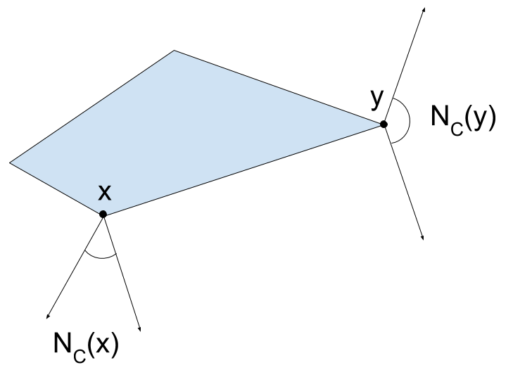
The normal cone is important for characterizing optimality in convex optimization: a point \(\bar{x}\) is optimal for the problem \(\min \{ f(x) : x \in C \}\) if and only if \(-\nabla f(\bar{x}) \in N_C(\bar{x})\). Indeed, if \(-\nabla f(\bar{x})\) were not in the normal cone, we could find \(x \in C\) such that \(-\nabla f(\bar{x})^T (x - \bar{x}) > 0\). This means that \(d = x-\bar{x}\) is a descent direction for \(f\) and moving in this direction maintains feasibibility.

The optimality condition \(-\nabla f(\bar{x}) \in N_C(\bar{x})\) is equivalent to the KKT conditions. (With the Lagrange multipliers giving the representation of \(-\nabla f(\bar{x})\) in the normal cone.) This is because for a convex set described by smooth inequalities \(g_1 \leq 0, \ldots, g_p \leq 0\), the normal cone at \(x\) is the cone generated by the gradients of the active constraints:

\[N_C(x) = \left\{ \sum_{i=1}^p \lambda_i \nabla g_i(x) : \lambda_i \geq 0, \ g_i(x) \lambda_i = 0 \right\}.\]

Convex congugates

Given a function \(f : \mathbb{R}^n \to \mathbb{R}\), the convex conjugate is defined by

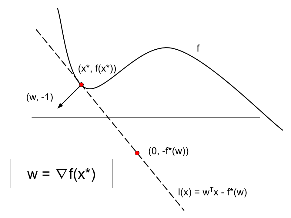
\[f^*(w) = \sup_{x \in \mathbb{R}^n} w^T x - f(x).\]

The function \(f^*\) is convex, even if \(f\) is not (since it is the pointwise maximum of convex functions).

Notice that \(f^*(w)\) is the is the smallest offset \(b\) so that \(l(x) = w^T x - b\) globally underestimates \(f\). Geometrically this defines a nonvertical supporting hyperplane \(H_w = \{ (x,y) : y = w^T x - f^*(w) \}\) to the graph of \(f\) that intersects the vertical axis at \(-f^*(w)\).

Also note that \(f^*(w)\) is the maximum value of the linear functional \((x, y) \mapsto (w, -1)^T (x,y)\) over the graph of \(f\), and so \((w,-1)\) is normal to the graph of \(f\) where the hyperplane \(H_w\) touches:

\[\begin{aligned} f^*(w) &= \sup_{x \in \mathbb{R}^n} w^T x - f(x) \\ &= \sup_{x \in \mathbb{R}^n} (w, -1)^T (x, f(x)) \\ &= \sup_{(x,y) \in \text{grh}(f)} (w, -1)^T (x,y). \end{aligned}\]

We can replace the graph with the epigraph since

\[\sup_{(x,y) \in \text{grh}(f)} (w, -1)^T (x,y) = \sup_{(x,t) \in \text{epi}(f)} (w, -1)^T (x,t).\]

(Recall that the graph of a function is the set \(\text{grh}(f) = \{ (x, y) : x \in \mathbb{R}^n, y = f(x) \}\) and the epigraph is the region “above” the graph \(\text{epi}(f) = \{ (x, t) : x \in \mathbb{R}^n, t \geq f(x) \}\).)

There is thus a correspondence between the domain of \(f^*\) and supporting hyperplanes to the epigraph of \(f\).

Biconjugate

A “dual” view of \(f\) is given by the pointwise maximum of all linear underestimators:

\[\phi(x) = \sup \{ l(x) : l \text{ is a linear underestimator of f} \}.\]

In fact, if \(f\) is closed and convex, then \(\phi = f^{**}\), the biconjugate of f. Geometrically it is clear that

\[f^{**}(0) = \sup_w -f^*(w) = \phi(0)\]

from the previous discussion, and the same geometry applies at other points.

Value function and the Lagrange dual

Consider the primal optimization problem

\[\begin{aligned} \inf_{x \in E} &\quad f(x) \\ \text{subject to} &\quad g(x) \leq 0, \end{aligned}\]

where \(f : E \to \mathbb{R}\) is the objective and \(g : E \to \mathbb{R}^p\) are contraint functions. The value function describes how the optimal value changes as constraints are relaxed:

\[v(b) = \inf \{ f(x) : x \in E,\ g(x) \leq b\}.\]

The conjugate of the value function closely related to the Lagrange dual:

\[\begin{aligned} v^*(w) &= \sup_{b \in \mathbb{R}^p} \left\{ w^T b - v(b) \right\} \\ & = \sup_{b \in \mathbb{R}^p,\ x \in E,\ g(x) \leq b} \left\{ w^T b - f(x) \right\} \\ & = \sup_{s \geq 0,\ x \in E} \left\{ w^T (g(x) + s) - f(x) \right\} \\ & = \sup_{x \in E} \left\{ w^T g(x) - f(x) \right\} + \sup_{s \geq 0} w^T s \\ &= -\inf_{x \in E} \left\{ f(x) + (-w)^T g(x) \right\} + \sup_{s \geq 0} w^T s \\ &= \left\{ \begin{matrix} -\Pi(-w) &\quad w \leq 0 \\ \infty &\quad \text{otherwise} \end{matrix} \right. \\ &= -\Pi(-w). \end{aligned}\]

The above relation shows that the Lagrange dual problem can be viewed as maximization over supporting hyperplanes to the value function. From previous discussions, it is clear that \(v^{**}(0)\) is the dual optimal value and \(v(0)\) is the primal optimal value. The dual optimal vectors are subgradients to the value function at 0 and therefore contain information about how sensitive the optimal value is to the constraints.

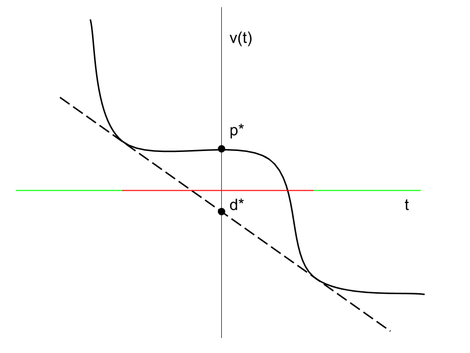
The figure above shows a duality gap (\(p^* > d^*\)) for the original problem \(v(0)\). Some of the peturbed problems \(v(t)\) have duality gaps (red regions) and others do not (green regions).

There is no duality gap if \(v\) has a nonvertical supporting hyperplane at 0. This is true when \(f\) and each component of \(g\) is convex and Slater’s condition holds: there is a point \(x\) so that \(g(x) < 0\). Convexity is not sufficient to ensure no duality gap; the function \(v\) must also be closed at 0 (see the figure below).

The value function above corresponds to the following convex program (which fails Slater’s condition):

\[\begin{aligned} \inf_{x, y > 0} &\quad e^{-x} \\ \text{subject to} &\quad x^2 / y \leq 0. \end{aligned}\]

Fenchel duality

Fenchel duality consists of the primal problem

\[\inf_x \{ f(x) + g(Ax) \}\]

and the dual problem

\[\sup_w \{ -f^*(A^Tw) - g^*(-w) \}.\]

Duality is analyzed through the perturbation function \(v(u) = \inf_x \{ f(x) + g(Ax - u) \}\), which is convex in \(u\).

Notice that the primal optimal value is \(v(0)\), and the dual problem is \(\max_w -v^*(w) = v^{**}(0)\) since:

\[\begin{aligned} -v^*(w) &= \inf_u \{ v(u) - w^T u \} \\ &= \inf_{u,x} \{ f(x) + g(Ax-u) - w^Tu \} \\ &= \inf_{z,x} \{ f(x) + g(z) - w^T(Ax - z) \} \\ &= \inf_{z,x} \{ f(x) - (A^Tw)^T x + g(z) - (-w)^T z \} \\ &= -f^*(A^T w) - g^*(-w). \end{aligned}\]

Strong duality holds when 0 belongs to the interior of the domain of \(v\) (recall the domain of convex function is the region where it is not positive infinity). Further note that:

\[\begin{aligned} u \in \text{dom} (v) &\iff \exists x \text{ s.t } f(x) + g(Ax - u) < \infty \\ &\iff \exists x \text{ s.t } x \in \text{dom}(f) \text{ and } Ax - u \in \text{dom}(g) \\ &\iff u \in A \text{dom}(f) - \text{dom}(g), \end{aligned}\]

so \(\text{dom}(v) = A \text{dom}(f) - \text{dom}(g)\), and strong duality holds if \(0 \in \text{int}(A \text{dom}(f) - \text{dom}(g))\).

Duality via perturbation functions

We derived both Lagrangian and Fenchel duality by reasoning about perturbations. More generally a perturbation function \(F(x,u)\) is one where \(f(x) = F(x,0)\). By considering

\[v(u) = \inf_x F(x, u)\]

and its conjugate

\[\begin{aligned} -v^*(w) &= \inf_u \{ v(u) - w^T u \} \\ &= \inf_{x,u} \{ F(x,u) - w^T u \} \\ &= \inf_{x,u} \{ F(x,u) - (0,w)^T (x,u) \} \\ &= -F^*(0,w) \end{aligned}\]

we get the primal problem

\[\inf_x F(x,0)\]