Propagation of error

Propagation of error describes how uncertainty in estimates propagates forward when we consider functions of those estimates.

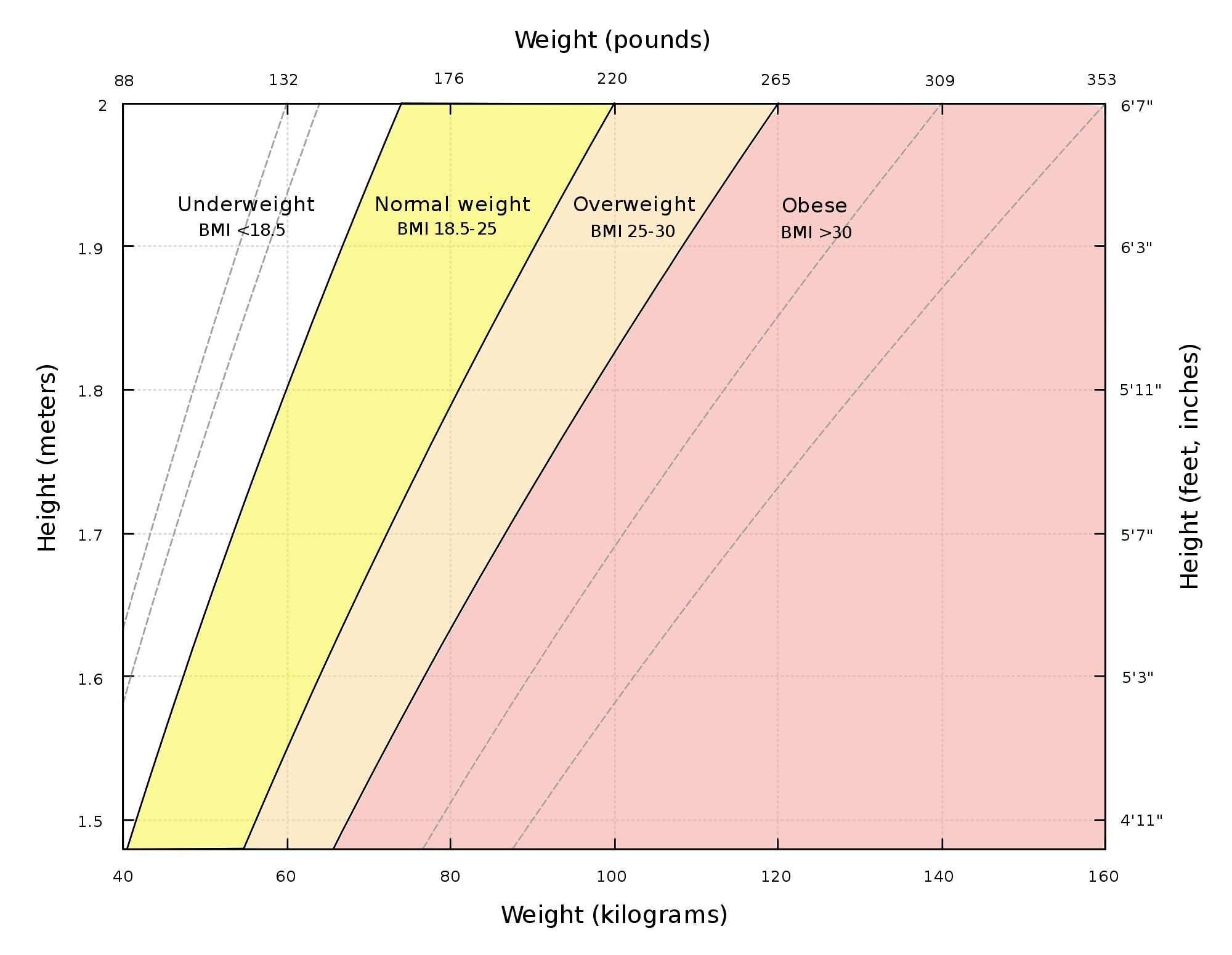
Suppose I have height and weight measurements for a sample of people.  What is the mean and variance of the BMI?  (BMI is 703 times the weight (in pounds) over the square of the height (in inches).)

The obvious thing is to compute the BMI for each individual in the data set, and then compute the mean of and variance of the BMIs.  But suppose that I don’t have access to the original data, but only have summary statistics about the heights and weights.  What can I say about BMI then?

Propagation of error is derived by taking a first-order Taylor expansion about the mean.  Suppose \(X\) is a random variable with mean \(\mu\) and variance \(\sigma^2\), and we want to approximate the mean and variance of \(f(X)\).  We know \(f(X) \approx f(\mu) + f'(\mu)(X- \mu)\), so

\[\begin{aligned} \textbf{E}(f(X)) &\approx \textbf{E}(f(\mu) + f'(\mu)(X- \mu)) = f(\mu) \\ \textbf{Var}(f(X)) &\approx \textbf{Var}(f(\mu) + f'(\mu)(X- \mu)) = f'(\mu)^2 \textbf{Var}(X). \end{aligned}\]

As a sanity check, notice that \(\textbf{Var}(f(X))\) is modulated by \(\vert f'(\mu)\vert\).  This makes sense: if \(f\) is flat near \(\mu\), the “range” of \(X\) is compressed (less variation), and if \(f\) is steep, the “range” is expanded (more variation).  How good are these approximations?  This depends on how non-linear \(f\) is and how central \(X\) is about its mean.  But the approximations are good enough for the central limit theorem.

Consider a central limit theorem type statement like \(\sqrt{n} (X_n - \theta)\) converges to \(N(0, \sigma^2)\) in distribution (this is the central limit theorem if \(X_n\) is the sample mean of \(n\) data points and \(\theta\) is the true mean.)  If we consider some function of \(X_n\), we still have a limit theorem:  \(\sqrt{n} (f(X_n) - f(\theta))\) converges to \(N(0, f'(\theta)^2 \sigma^2)\) (provided the derivative is non-zero).  The proof is just a Taylor expansion about \(\theta\):

\[\begin{aligned} \sqrt{n} (f(X_n) - f(\theta)) &= \sqrt{n} (f(\theta) + f'(\theta)(X_n - \theta) + \epsilon - f(\theta)) \\ &= f'(\theta) \sqrt{n} (X_n - \theta) + \sqrt{n} \epsilon \end{aligned}\]

The first term \(f'(\theta) \sqrt{n} (X_n - \theta)\) converges in distribution to \(f'(\theta) N(0, \sigma^2) = N(0, f'(\theta)^2 \sigma^2)\).  The error \(\sqrt{n} \epsilon\) converges to 0 in probability.  I think the easiest way to see this is to write \(\sqrt{n} \epsilon\) as \(\vert \sqrt{n} (X_n - \theta)\vert   \cdot \left(\epsilon / \vert X_n - \theta\vert \right)\).  The first factor \(\vert \sqrt{n} (X_n - \theta)\vert\) converges in distribution to the absolute value of a normal random variable, and the second factor \(\epsilon / \vert X_n - \theta\vert\) converges to 0 in probability.

Using a multivariate Taylor expansion, we have the same statements in higher dimensions: if \(\sqrt{n} (X_n - \theta)\) converges in distribution to a multivariate normal \(N(0, \Sigma)\), then \(\sqrt{n}(f(X_n) - f(\theta))\) converges to a univariate normal \(N(0, \nabla f(\theta)^T \Sigma \nabla f(\theta))\).  Let’s work through the height, weight, and BMI example to make this more concrete.

Suppose we have summary statistics about the weights and heights: \(\mu_w = 164.39\), \(\sigma_w = 23.58\),  \(\mu_h = 70.45\), \(\sigma_h = 3.03\), and correlation \(\rho = 0.40\).  Let \(f(w, h) = 703 w / h^2\) be the BMI. The covariance matrix and gradient at the mean are:

\[\begin{aligned} \Sigma &= \begin{bmatrix} \sigma_w^2 & \rho \sigma_w \sigma_h \\ \rho \sigma_w \sigma_h & \sigma_h^2 \end{bmatrix} =\begin{bmatrix} 556.02 & 28.58 \\ 28.58 & 9.18 \end{bmatrix} \\ \nabla f(\theta) &= 703 \begin{bmatrix} 1/\mu_h^2 \\ -2 \mu_w / \mu_h^3 \end{bmatrix} = \begin{bmatrix} 0.14 \\ -0.66 \end{bmatrix}. \end{aligned}\]

By propagation of error combined with the central limit theorem, the mean BMI of \(n\) people is approximately normally distributed with mean \(f(\theta) = (703)(164.39) / (70.45^2) = 23.28\) and variance \(\nabla f(\theta)^T \Sigma \nabla f(\theta)) / n = 9.82 / n\).  The approximation is better the larger \(n\) is.

Written on April 28th, 2018 by Scott Roy