Sampling from distributions

There is almost no difference between knowing a distribution’s density (and thus knowing its mean, variance, mode, or anything else about it) and being able to sample from the distribution.  On the one hand, if we can sample from a distribution, we can estimate the density with a histogram or kernel density estimator.  Conversely, I’ll discuss ways to sample from a density in this post.

I said “almost no difference” because to sample from a density, you do need some external source of randomness.  Sampling techniques do not create randomness, but rather transform one kind of random samples (usually uniform) into samples from a specified density.  As an aside, a uniform random sample $x$ can be generated by flipping a coin infinitely many times.  First flip a coin to decide whether to look for $x$ in the first or second half of the interval $(0,1)$.  If the coin shows heads, we look for $x$ in $[0,0.5)$, otherwise we look in $[0.5,1)$.  This process is repeated recursively.  For example, if the first toss is heads, we toss again to decide whether to look for $x$ in $[0,0.25)$ or $[0.25,0.5)$.  In practice, to sample $x$ with 9 digits of accuracy, we only need to toss the coin 30 times.

The observation that we can estimate anything about a distribution by being able to draw samples from it is important for Bayesian statistics in practice.  Bayesian inference is a matter of being able to draw from the posterior.  I’ll now touch on various methods for generating random samples from a given density.

Use related distributions

There are many relationships between common random variables.  For example,

• If $Z$ is standard normal, then $\sigma Z + \mu$ is $N(\mu, \sigma^2)$.
• If $Z$ is standard normal and $V$ is independently $\chi^2_{p}$, then $T = \frac{Z}{\sqrt{V / p}}$ has Student’s t-distribution with $p$ degrees of freedom.
• If $U$ is uniform, then $-\frac{1}{\beta} \log(U)$ is exponential with rate $\beta$.
• If $X \sim \text{Gamma}(\alpha, \lambda)$ and independently $Y \sim \text{Gamma}(\beta, \lambda)$, then $\frac{X}{X+Y} \sim \text{Beta}(\alpha, \beta)$.

These relationships can be exploited to generate random samples.  For example, to draw $x$ from an exponential distribution with rate parameter 1, first draw $u$ uniformly over $(0,1)$ and set $x = -\log(u)$.  Along the same line, a $\text{Beta}(\alpha, \beta)$ random draw can be formed as the ratio of two exponential draws (exponential is a special case of gamma):

$$\frac{\frac{1}{\alpha}\log(u_1)}{\frac{1}{\alpha}\log(u_1) + \frac{1}{\beta}\log(u_2)}$$

Inverse CDF method

If $F$ is an invertible CDF and $U$ is uniform, then $X = F^{-1}(U)$ is distributed with CDF $F$:

$$\begin{aligned} \textbf{P}(X \leq t) &= \textbf{P}(F^{-1}(U) \leq t) \\ &=\textbf{P}(U \leq F(t)) \\ &= F(t) \end{aligned}$$

Summary: if we know the inverse CDF of a distribution, we can sample from it.  As an aside, the inverse CDF of an exponential distribution is $F^{-1}(t) = -\frac{1}{\beta} \log(t)$, which we used in the previous section.

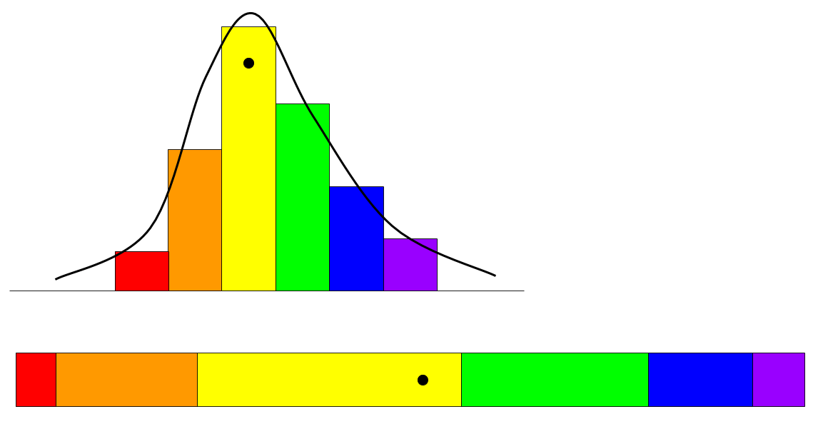
We can approximate the inverse CDF method with a Riemann sum.  Below I approximate a density with rectangles.

The CDF is represented by stacking these rectangles end to end to form a strip.  The inverse is represented in the color-coding.  In the figure, a dot is drawn uniformly on the strip, and is mapped back (using colors) to get a sample from the density.

Rejection sampling

Rejection sampling is a technique to sample from a subset, assuming we know how to sample from the larger set.  I’ll explain the technique with an example.  Suppose I want to sample a random point from a lightning bolt subset of a square.

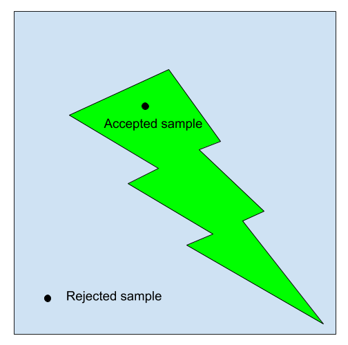
In rejection sampling, I first draw a point uniformly at random from the square, and I accept the sample if it lands in the lightning bolt, and reject the sample otherwise.  The accepted samples are distributed uniformly over the lightning bolt.The probability that a sample is accepted is the area of the lightning bolt over the area of the square.  The acceptance probability measures the efficiency of the method: if I want $n$ random samples from the lightning bolt, on average I have to draw $\frac{n}{\textbf{P}(\text{acceptance})}$ samples from the square.

Rejection sampling is often introduced as a technique for drawing from a density.  Drawing from a density is equivalent to drawing uniformly from the region below the density.  To be more precise, drawing a random variable from a density $f$ is equivalent to drawing uniformly from the region below the density in the following sense:

• If $(x,y)$ is drawn uniformly over the region below the density, then $x$ is a random draw from $f$.
• If $x$ is a random draw from $f$, and $y$ is a uniform draw from the interval $(0, f(x))$, then $(x, y)$ is uniformly distributed over the region below the density.

To sample from $f$ with rejection sampling, we first find a proposal density $g$ and constant $c \geq 1$ with $cg \geq f$. We then

1. Sample from $g$ to construct a uniform sample under $c g$.
2. Apply rejection sampling to get a uniform sample under $f$.
3. The x-coordinate of the uniform sample under $f$ is a sample from $f$.

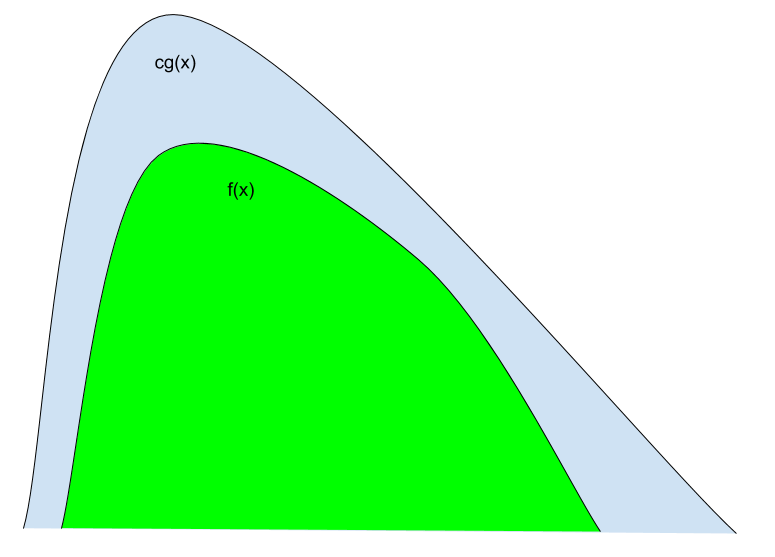
The acceptance rate is $1/c$, the area under $f$ over the area under $cg$.  The more $g$ is like $f$, the more efficient the rejection sampling algorithm.

Constructing a proposal density $g$ that is 1) easy to sample from and 2) closely resembles $f$ can be challenging.  Let’s walk through an example with the standard normal density $f(x) = \frac{1}{\sqrt{2\pi}} e^{-x^2/2}$.  Since $f$ is log-concave, we can construct a piecewise exponential curve $g$ that upper bounds (and well approximates) $f$.  This piecewise exponential curve can be sampled from quickly using the inverse CDF method.

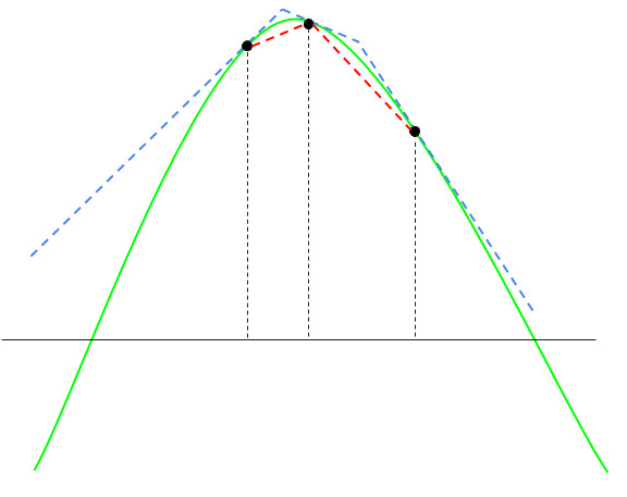
Adaptive rejection sampling

Adaptive rejection sampling is a variant of rejection sampling that learns the proposal density $g$ as it runs.  The method applies to log-concave densities and constructs a piecewise exponential $g$ by constructing a piecewise linear function that approximates (and upper bounds) $h(x) = \log f(x)$.

Issues in high dimensions

Rejection sampling is generally inefficient in high dimensions.  To explain, suppose I sample from standard normal by using a normal with variance $\sigma^2 \geq 1$ as the proposal density.  (This example is just to illustrate a point.  We can get a standard normal sample from any other normal sample by “standardizing,” and do not need to use rejection sampling.)  The standard normal has density $f(x) = \frac{1}{\sqrt{2\pi}} e^{-x^2/2}$ and the proposal density is $g(x) = \frac{1}{\sqrt{2\pi} \sigma} e^{-x^2/(2\sigma^2)}$.  Suppose $\sigma = 1.001$.  In this case, we can set $c = \sigma$ so that $cg \geq f$ and the acceptance probability is $1 / c \approx 99.9\%$.  Now let $f$ be the density of a 5000-dimensional normal random vector with covariance matrix $I$ and suppose $g$ has covariance matrix $\sigma^2I$.  In this case $c = \sigma^{5000}$ and the acceptance rate $1 / c$ is less than a percent.

In high dimensional problems that arise in Bayesian sampling, methods based off Markov chains such as MCMC or Gibbs sampling are used.

References

• Adaptive Rejection Sampling for Gibbs Sampling by W. R. Gilks and P. Wild

Written on May 12th, 2018 by Scott Roy