statsandstuff a blog on statistics and machine learning
ROC space and AUC
Before discussing ROC curves and AUC, let’s fix some terminology around the confusion matrix:
- Condition positive (negative): real positive (negative) case in the data
- True positive (negative): condition positive (negative) that is classified as positive (negative)
- False positive (negative): condition negative (positive) that is classified as positive (negative)
- True positive rate (TPR): empirically defined as (# true positives) / (# condition positives). More generally, it is the probability that a condition positive is labelled as positive.
- False positive rate (FPR): empirically defined as (# false positives) / (# condition negatives). More generally, it is the probability that a condition negative is classified as positive.
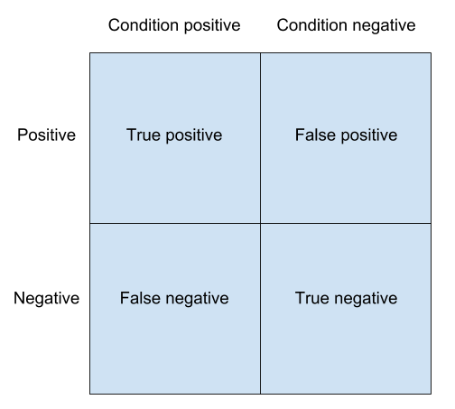
True positive rate and false positive rate do not depend on the class ratio, that is, the ratio of condition positives to condition negatives in the data. Contrast this with precision, the number of true positives over the number of predicted positives, which does depend on the class ratio.
ROC Space
The concept of ROC (receiver operator characteristic) space was introduced by engineers during WWII. Radar operators had to decide if a blip on a radar screen was an enemy target or not. The performance of different operators can be compared by plotting an operator’s true positive rate along the y-axis and false positive rate along the x-axis.
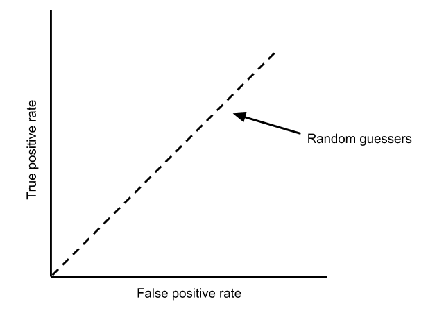
In “ROC space,” the better operators are in the upper, left corner (high true positive rate, low false positive rate). Any decent operator lies in the upper, left region above the diagonal. In fact, points on the diagonal correspond to the performance of “random guessers.” Suppose Jim flips a coin and classifies a blip as an enemy target if the coin shows heads. In this case, Jim will classify half of condition positives as targets (50% true positive rate) and half of condition negatives as targets (50% false positive rate). If the coin is biased and has a 70% chance of showing heads, Jim’s TPR and FPR will both be 70%. The entire diagonal line corresponds to the performance of random guessers who use biased coins with varying probabilities of showing heads.
ROC Curves
Like radar operators, we can compare the performance of classifiers by plotting TPR and FPR in ROC space. Before discussing ROC curves, I want to distinguish between a classifier and a scorer. A classifier labels an input as positive or negative. Its output is binary. Many classifiers in machine learning are built from scorers. A scorer assigns each input a score that measures a “belief” that the input is a positive example. For example, a logistic regression scorer assigns each input a probability score of being a positive example. (As an aside, the probability scores computed by logistic regression (or any machine learning model) need not be well-calibrated, true probabilities. For this reason, care should be taken when comparing scores from different models.) We get a logistic regression classifier, for example, by labelling an input as positive if its score is greater than 0.5. A scorer generates many classifiers indexed by a threshold \(t\), where the classifier at threshold \(t\) labels an input as positive or negative depending on if its score is above or below \(t\).
We can plot the performance of all the classifiers generated by a scorer in ROC space. For high values of \(t\), few examples are classified as positive, and so both the true positive rate and false positive rate are low. Similarly, the true positive rate and false positive rate are are high for low values of \(t\). So the ROC curve for a scorer starts in the upper right corner, ends in the lower left corner, and will (hopefully) bulge out toward the upper left corner.
AUC
A good scorer will have an ROC curve that bulges out toward the upper left corner. The AUC is the area under the ROC curve, and is a heuristic for measuring how much the curve bulges toward the upper left corner. A perfect scorer has AUC 1.
AUC has an alternative interpretation: it is the probability that a condition positive has a higher score than a condition negative. Let’s see why. Let \(\beta(t)\) be the TPR at threshold \(t\) and \(\alpha(t)\) be the FPR at threshold \(t\). (Notice that the use of \(\alpha\) and \(\beta\) here is consistent with their use to denote Type I error and power in statistics.) Let \(f_{+}(x)\) be the score density of the condition positives. Then we can write \(\beta(t) = \int_{t}^{\infty} f_{+}(x)\ dx\). Similarly, \(\alpha(t) = \int_t^{\infty} f_{-}(x) \ dx\). The AUC is the integral over infinitesimal rectangles under of the ROC curve. The rectangle at \(\alpha\) has height \(\beta(t)\) and width \(d\alpha = f_{-}(t) dt\).
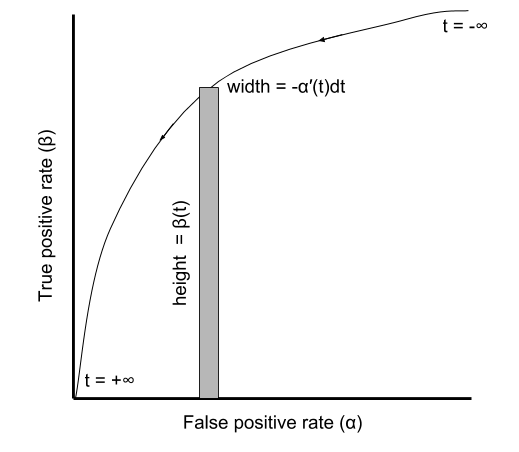
Putting things together, we have
\[\begin{aligned}\text{AUC} &= \int \beta(t) f_{-}(t) dt \\ &= \int \textbf{P}(\text{condition positive has score greater than } t)\ \textbf{P}(\text{condition negative has score } t) dt \\ &= \textbf{P}(\text{condition positive has higher score than condition negative}). \end{aligned}\]ROC curves and AUC (being based on TPR and FPR) do not depend on the class ratio in the data.
Picking the “best” classifier in ROC space
A classifier above and to the left of another in ROC space is objectively better. But not all points in ROC space are comparable.
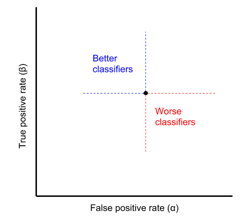
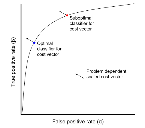
For example, a classifier can have a better TPR than another, but a worse FPR. Choosing between incomparable classifiers depends on the specific problem. In particular, it depends on the cost of a false positive, the cost of a false negative, and the ratio of condition positives to condition negatives in the data. As an example, consider a classifier that predicts if a patient has HIV. In this case, the cost of a false negative (failing to detect an HIV positive patient) is significantly more than the cost of a false positive (incorrectly diagnosing HIV).
Let’s model expected total cost. Each mistake has a cost. Let \(M_{+}\) be the number of false positives and \(c_{+}\) be the cost of a false positive (with similar definitions for \(M_{-}\) and \(c_{-}\)). In expectation, \(M_{+}\) is \(n p_{-} \alpha\), where \(n\) is the number of classified points, \(p_{-}\) is the probability of a condition negative, and \(\alpha\) is the true positive rate. Similarly, the expected value of \(M_{-}\) is \(n p_{+} (1-\beta)\). The average total cost is
\[c_{+} n p_{-} \alpha + c_{-} n p_{+} (1-\beta),\]and we can find the best classifier by minimizing this over ROC space. Equivalently, we can maximize the linear functional
\[(\alpha, \beta) \mapsto -\left( \frac{c_{+}}{c_{-}} \right) \left( \frac{p_{-}}{p_{+}} \right) \alpha + \beta.\]Notice that the selection of the best classifier only depends on the cost ratio \(c_{+} / c_{-}\) and the class ratio \(p_{-} / p_{+}\). In the special case where the classes are balanced and a false positive has the same cost as a false negative, the best classifier is the one furthest in the northeast direction.

Interpolating classifiers in ROC space
Given any two classifiers in ROC space, we can interpolate on the line segment between them. Suppose classifier 1 is at \((\alpha_1, \beta_1)\) and classifier 2 is at \((\alpha_2, \beta_2)\). We can form a combined classifier that lies at \((\theta \alpha_1 + (1-\theta) \alpha_2, \theta \beta_1 + (1-\theta) \beta_2)\) as follows. We flip a coin that shows heads with probability \(\theta\) and predict the output of classifier 1 if the coin shows heads, and predict the output of classifier 2 if the coin shows tails. In this way, we can get the performance of any point in the convex hull of the classifiers we plot in ROC space.
References
- Measuring classifier performance: a coherent alternative to the area under the ROC curve by David J. Hand
- An introduction to ROC analysis by Tom Fawcett