statsandstuff a blog on statistics and machine learning
Controlling error when testing many hypotheses
In a hypothesis test, we compute some test statistic \(T\) that is designed to distinguish between a null and alternative hypothesis. We then compute the probability p(T) of observing a test statistic as large or more extreme as T under the null hypothesis, and reject the null hypothesis if the p-value p(T) is sufficiently small. (As an aside, the p-value can alternatively be viewed as the probability, under the null hypothesis, of observing data as rare or rarer than the data we actually saw. This perspective does not require coming up with a test statistic first.)
When we perform many tests (for example, testing association with disease on thousands of genes), we are likely to get false positives, even if each individual test has a small probability of error (see Multiple hypothesis tests). With careful analysis, though, we can understand (and therefore control) the number of false positives our battery of tests yields.
The most important insight into analyzing the “multiple testing problem” is the observation that under the null hypothesis, the p-values are uniformly distributed. To see this, suppose that under the null, the test statistic is distributed \(T \sim f\). The p-value \(p(T)\) is at most \(\alpha\) if the test statistic \(T\) falls in the \(\alpha\)-tail of the distribution \(f\). By definition, this happens with probability \(\alpha\), and so \(\textbf{P}(p(T) \leq \alpha) = \alpha\) and \(p(T) \sim \text{Uniform}(0,1)\). (This is more or less the same reasoning used in the inverse CDF method; see Sampling from distributions.)
Throughout we assume that we test \(m\) independent hypotheses, \(m_0\) of which are null and \(m_1 = m - m_0\) of which are alternative. We do not know the number of null hypotheses \(m_0\) a priori. (If \(m_0\) is large, we can estimate it from a p-value histogram because \(m_0\) of the p-values are uniformly distributed.) We reject a hypothesis if its p-value is less than some threshold \(t\). We let V denote the number null hypotheses we rejected.
Bonferroni correction
The Bonferroni correction sets a rejection threshold \(t\) so that the probability of having a false positive is controlled at level \(\alpha\): \(\textbf{P}(V \geq 1) \leq \alpha\). At significance level \(t\), what is the probability that we reject some null hypothesis? It is easier to compute the probability of the complement event that we do not reject any null hypotheses. This happens if \(m_0\) i.i.d. uniform p-values land in the interval \([t,1]\), which occurs with probability \((1-t)^{m_0}\). We thus have:
\[\begin{aligned} \textbf{P}(V \geq 1) = 1 - (1-t)^{m_0} \leq \alpha \quad &\Leftrightarrow \quad t \leq 1 - (1-\alpha)^{1/m_0}. \end{aligned}\]The threshold \(t(\alpha) = 1 - (1-\alpha)^{1/m_0}\) caps the family-wise error rate (FWER) \(\textbf{P}(V \geq 1)\) at \(\alpha\). We do not know \(m_0\) a priori, but replacing \(m_0\) with \(m\) only makes the threshold smaller, and therefore still controls the FWER. If we have a better upper estimate of \(m_0\) (from a histogram of p-values, for example), we can use it instead of \(m\).
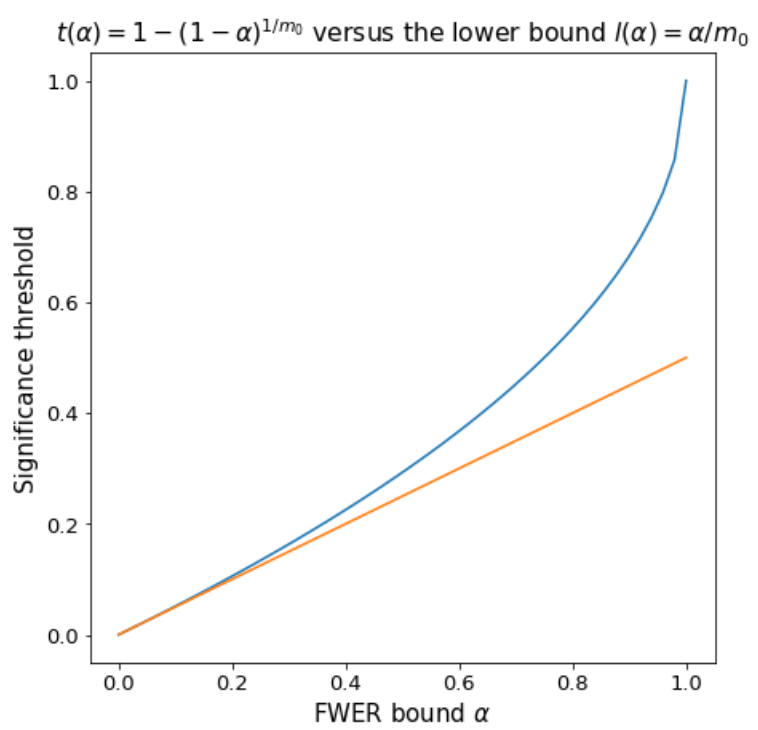
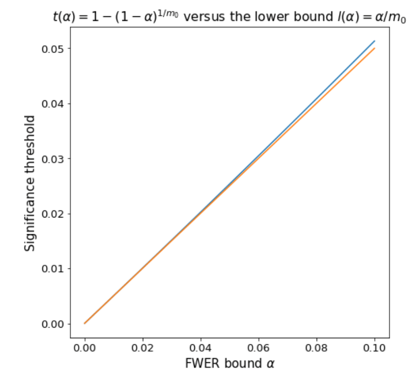
The formula for the threshold \(t(\alpha)\) is quite ugly, but is convex and can therefore be underestimated with its tangent line \(l(\alpha) = \alpha/m_0\) at \(\alpha=0\). The approximation is near perfect for practical values of \(\alpha \leq 0.1\).
 |
 |
The Bonferroni correction controls the FWER at \(\alpha\) and then tests for significance at level \(\alpha/m\) (it is usually proved in a simpler way using a union bound). For a large numbers of tests, the Bonferroni correction is too strict and often results in no positive findings.
A slight improvement that still controls the FWER at level \(\alpha\) is the Holm-Bonferroni method. This procedure gradually increases the significance level. The smallest p-value \(p_{(1)}\) is tested at threshold \(\alpha / m\) (the same as the Bonferroni method), but the next smallest p-value \(p_{(2)}\) is tested with threshold \(\alpha / (m-1)\), and the next smallest is tested at level \(\alpha / (m-2)\), and so on. The procedure stops when a p-value is not rejected. The Holm-Bonferroni method is still very strict when \(m\) is large. (Both the Bonferroni method and the Holm-Bonferroni procedure can be made more powerful by replacing \(m\) with a better overestimate of \(m_0\).)
The methods we discuss next allow some false positives, but control the number of false positives.
Controlling k-FWER
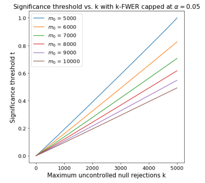
Suppose we’re willing to allow \(k\) false positives, but control the probability \(\textbf{P}(V \geq k+1)\) of having more than \(k\) false positives (called the k-FWER). Notice that we have more than \(k\) false positives if the \((k+1)\)th largest null p-value is less than the significance threshold \(t\). Since the null p-values are uniformly distributed, the \((k+1)\)th largest null p-value is distributed \(\text{Beta}(k+1, m_0 - k)\). We simply find the threshold \(t\) such that \(\textbf{P}( \text{Beta}(k+1, m_0 - k) \leq t) = \alpha\). Here is a plot.
Controlling the false discovery rate
Roughly speaking, the false discovery rate (FDR) is \(\textbf{P}(\text{test is null} \vert \text{test is rejected})\). This is the reverse of the false positive rate \(\textbf{P}(\text{test is rejected} \vert \text{test is null})\), the quantity that is traditionally controlled in hypothesis testing. Limiting the FDR and the FPR controls the number of false positives, but the denominators used to compute the two rates differ. The FDR uses the number of rejections in the denominator, whereas the the FPR uses the number of null tests. The difference between the two is much like the difference between precision and recall.
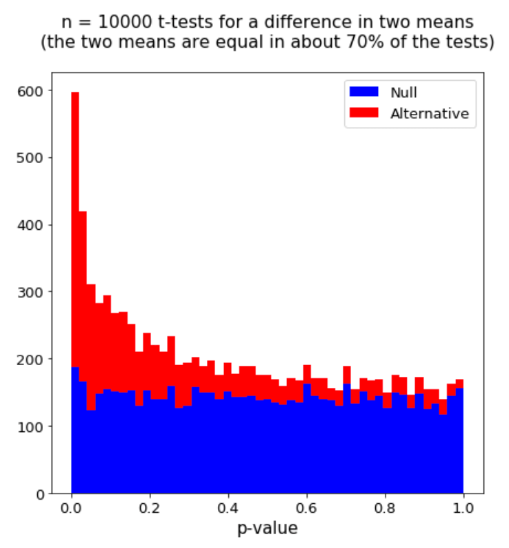
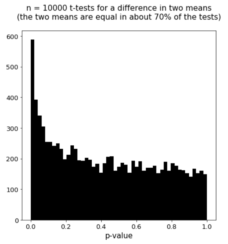
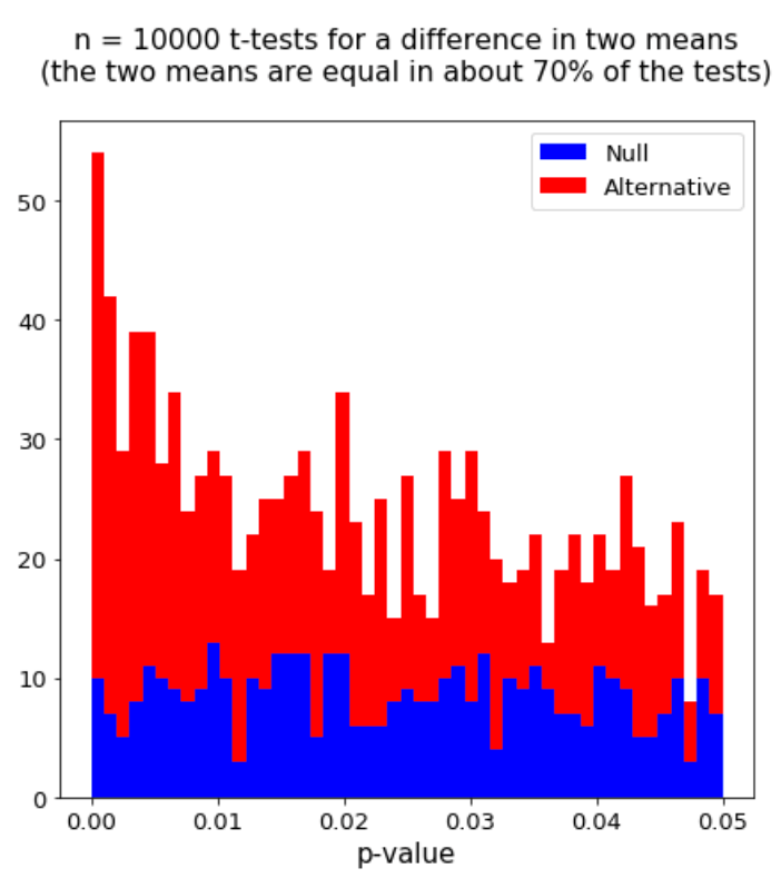
Below is the p-value histogram for 10,000 t-tests for a difference in two means. The two means were equal in about 70% of the tests (70% of the tests were null). The p-value distribution is a mixture of a uniform distribution (from the null tests) and a distribution concentrated near 0 (from the non-null tests). A priori we do not know which p-values correspond to the null tests (we observe the black histogram on the left); since this data is simulated, though, I show which p-values correspond to null tests in the red/blue histogram on the right.
 |
 |
The FDR at significance threshold \(t\) is the number of null p-values to the left of \(t\) over the total number of p-values to the left of \(t\) (the proportion of blue area to the left of \(t\) in the histogram.) In most cases, the FDR decreases with the significance threshold \(t\). Below we zoom in on the histogram in the \([0, 0.05]\) region.
A priori we do not know which p-values correspond to null tests (the blue portion of the p-value histogram). Nonetheless we can assume that all p-values bigger than, for example, 0.5 correspond to null tests. In this case, we estimate the number of null tests via the relation \(0.5 m_0 = \# \{ \text{p-values} \geq 0.5\}\), where \(m_0\) is the (unknown) number of null tests. Rather than use 0.5, we can parametrize with \(s\) and estimate the fraction of null tests \(\frac{m_0}{m}\) with \(\hat{\pi}_0(s) = \frac{\# \{ \text{p-values} \geq s\}}{s m}\). The estimate is best (but noisy) for values of \(s\) near 1 (\(s\) controls the bias-variance tradeoff). Here is a plot of \(\hat{\pi}_0(s)\) versus \(s\).

Storey and Tibshirani suggest fitting a weighted cubic spline to the curve \(s \mapsto \hat{\pi}_0(s)\) and evaluating the spline at 1.
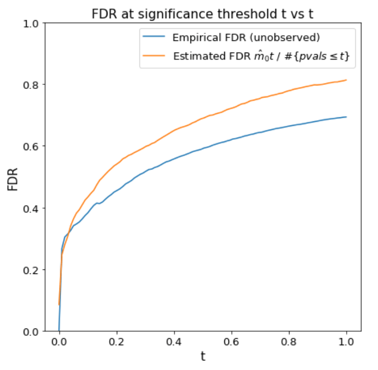
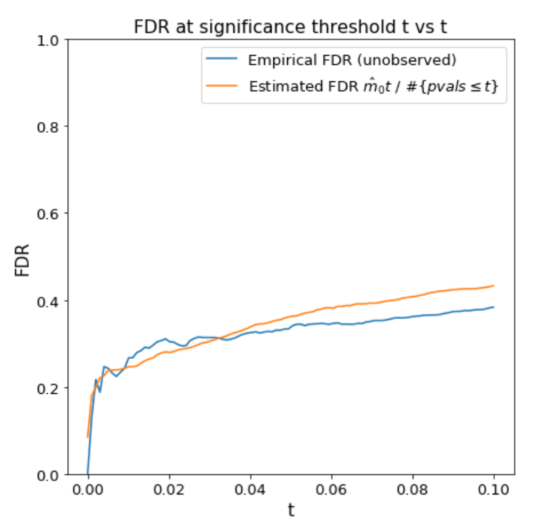
The estimated FDR at threshold \(t\) is
\[\begin{aligned} \text{FDR}(t) &= \frac{m \hat{\pi}_0 t}{\# \{ \text{p-values} \leq t\}}. \end{aligned}\]We plot this over \(t\).
 |
 |
Suppose we set \(t\) to the \(k\)th largest p-value \(p_{(k)}\) so that we reject the \(k\) smallest p-values. Then
\[\text{FDR}(p_{(k)}) = \frac{m \hat{\pi}_0 p_{(k)}}{k}.\]The q-value \(q_{(k)}\) corresponding to the \(k\)th largest p-value \(p_{(k)}\) is the smallest FDR you can get if you reject the first \(k\) p-values. In other words, it is
\[\begin{aligned} q_{(k)} &= \min_{j=k}^m \text{FDR}(p_{(j)}) \\ &= \min_{j=k}^m \frac{m \hat{\pi}_0 p_{(j)}}{j} \\ &= \min \left( \frac{m \hat{\pi}_0 p_{(k)}}{k},\ q_{(k+1)} \right), \end{aligned}\]where \(q_{(m+1)} = \infty\). To control the FDR at level \(\alpha\), we reject all hypotheses with q-value at most \(\alpha\). (The q-value gets its name from the fact that the letter q is a reflection of p and, roughly speaking, the q-value is \(\textbf{P}(\text{test is null} \vert \text{test is rejected})\) and the p-value is \(\textbf{P}(\text{test is rejected} \vert \text{test is null})\).)
The Benjamini-Hochberg procedure uses the same “q-values,” (discussed in Multiple hypothesis tests) but with the crude estimate \(\hat{\pi}_0 = 1\).
References
- Statistical Significance for Genome-Wide Experiments by Storey and Tibshirani
- The positive false discovery rate: A Bayesian interpretation and the q-value by Storey