statsandstuff a blog on statistics and machine learning
Inference based on entropy maximization

Entropy
For a discrete random variable, the surprisal (or information content) of an outcome with probability \(p\) is \(-\log p\). Rare events have a lot surprisal. For a discrete random variable with \(n\) outcomes that occur with probabilities \(p_1, \ldots, p_n\), the entropy \(H\) is the average surprisal
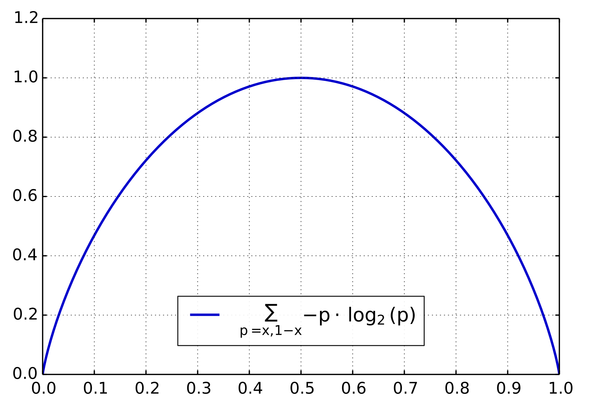
\[H(p_1,\ldots,p_n) = \sum_{i=1}^n -p_i \log p_i.\]Roughly speaking, entropy measures average unpredictability of a random variable. For example, the outcome of a fair coin has higher entropy (and is less predictable) than the outcome of a biased coin. Remarkably, the formula for entropy is determined (up to a multiplicative constant) by a few simple properties:
- Entropy is continuous.
- Entropy is symmetric, which means the value of \(H\) does not depend on the order of its arguments. For example, \(H(p_1,\ldots,p_n) = H(p_n, \ldots, p_1)\).
- Entropy is maximized when all outcomes are equally likely. For equiprobable events, the entropy increases with the number of outcomes.
- Entropy is consistent in the following sense. Suppose the event space \(\Omega\) is partitioned into sets \(\Omega_1, \ldots, \Omega_k\) that occur with probabilities \(\omega_j = \sum_{i \in \Omega_j} p_i\). Then total entropy is the entropy between the sets plus a weighted average of the entropies within each set: \(H(p_i : i \in \Omega) = H(\omega_1,\ldots, \omega_k) + \sum_{j=1}^k \omega_j H(p_i : i \in \Omega_j)\).
As an aside, variance behaves in the same way
\[\textbf{Var}(X) = \textbf{Var}(\textbf{E}(X\vert Y)) + \textbf{E}(\textbf{Var}(X\vert Y)),\]a relationship more apparent in the ANOVA setting (where \(X\) are measurements and \(Y\) are group labels): the total variation is the variation between groups plus the the average variation within each group.
Inference with insufficient data
Whether a good idea or not, we often want to make inferences with insufficient data. Doing so requires some kind of external assumption not present in the data. For example, L1-regularized linear regression solves under-determined linear systems by assuming that the solution is sparse. Another example is the principle of insufficient reason, which says that in the absence of additional information, we should assume all outcomes of a discrete random variable are equally likely. In other words, we should assume the distribution with maximum entropy.
Maximum entropy inference chooses the distribution with maximum entropy subject to what is known. As an example, suppose that the averages of the functions \(f_k\) are known:
\[\sum_{i=1}^n p_i f_k(x_i) = F_k.\]In this case, maximum entropy estimation selects the probability distribution that satisfies
\[\begin{aligned} \text{max.} &\quad -\sum_{i=1}^n p_i \log p_i \\ \text{s.t.} &\quad \sum_{i=1}^n f_k(x_i) p_i = F_k,\ 1 \leq k \leq K \\ &\quad \sum_{i=1}^n p_i = 1. \end{aligned}\]This convex problem has solution
\[p(x) = \frac{1}{Z} e^{\sum_{k=1}^K w_k f_k(x)},\]where \(Z\) and \(w_k\) are chosen so that the constraints are satisfied. (We use the notation \(p_i = p(x_i)\).) Notice that in this case, maximum entropy inference gives the same estimates of \(p_i\) that fitting an exponential family using maximum likelihood estimation gives.
Although maximum entropy estimation lets us answer a question such as “Given the mean of \(f(X)\), what is the mean of \(g(X)\)?”, we should always consider whether the answer is meaningful. For example, when \(f(x) = x\) and \(g(x) = x^2\), we are asking for the variance on the basis of just knowing the mean, and any a priori assumption that makes such a task feasible should be scrutinized.
References
- Information Theory and Statistical Mechanics by E. T. Jaynes
- Exercise 22.13 in Information Theory, Inference, and Learning Algorithms by David J. Mackay