statsandstuff a blog on statistics and machine learning
Introduction to neural networks
In this post, I walk through some basics of neural networks. I assume the reader is already familar with some basic ML concepts such as logistic regression, linear regression, and classifier decision boundaries.
Single neuron
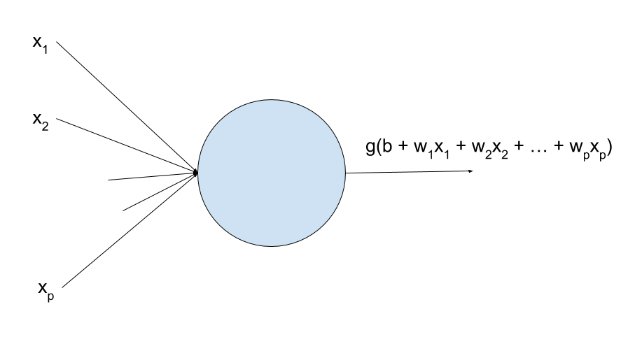
Neural networks are made up of neurons. A single neuron in a neural network takes inputs \(x_1, x_2, \ldots, x_p\), applies a linear transformation to these inputs to compute \(z = b + w_1 x_1 + \ldots + w_p x_p\), and then applies a (nonlinear) activation function to \(z\) to compute an output \(a = g(z)\).
Different activation functions result in different generalized linear models. For example, if \(g(z) = 1 / (1 + e^z)\) is the sigmoid function (also called the logistic function), the neuron is essentially a logistic regression, provided we fit the model using cross-entropy loss/maximum likelihood estimation. Similarly, if \(g(z) = z\) is the identity function, the neuron is a linear regression as long as we fit the model using square loss. Popular activation functions are
- sigmoid (\(g(z) = 1 / (1 + e^{-z})\))
- tanh (\(g(z) = (e^z - e^{-z}) / (e^{z} + e^{-z})\))
- RELU (\(g(z) = \max(0, z)\))
The tanh (plotted below) and sigmoid functions have the same shape, but the sigmoid takes values in \((0,1)\), whereas tanh takes values in \((-1,1)\). The precise relationship between the two is given by \(\tanh(z) = 2\text{sigmoid}(2z) - 1\).

A single neuron divides space with a hyperplane and can therefore learn to classify linearly separable data. As an example, consider a two dimensional feature space and a single neuron with a hyperbolic tangent activation function. The output of the neuron is
\[a = \tanh(w_1 x_1 + w_2 x_2 + b).\]Notice the neuron fires \(a = 0\) on the decision boundary \(w_1 x_1 + w_2 x_2 + b = 0\), is positive on one side of the boundary, and is negative on the other. By multiplying \(w_1\), \(w_2\), and \(b\) by a sufficiently large scalar, the boundary \(w_1 x_1 + w_2 x_2 + b = 0\) remains the same, but the transition from \(a = -1\) to \(a = 1\) as you move across the boundary essentially becomes a step function so that \(a = -1\) on one side, \(a = 0\) on the boundary, and \(a = 1\) on the other side.
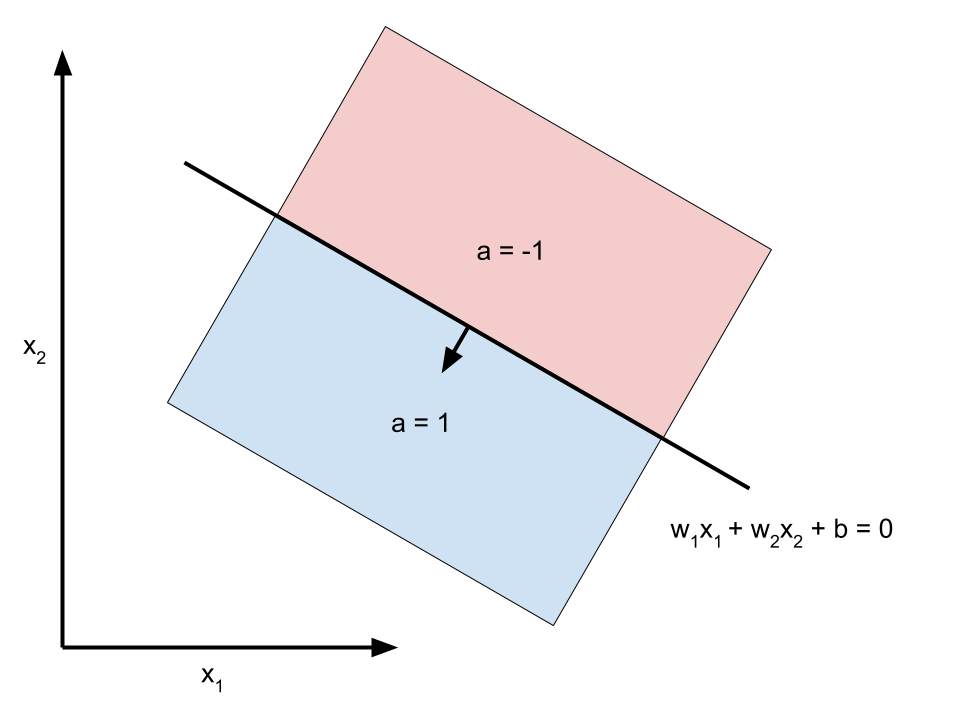
The key point is that one neuron can divide the plane in two. We use this observation later when we discuss decision boundaries of neural networks.
Neural network overview
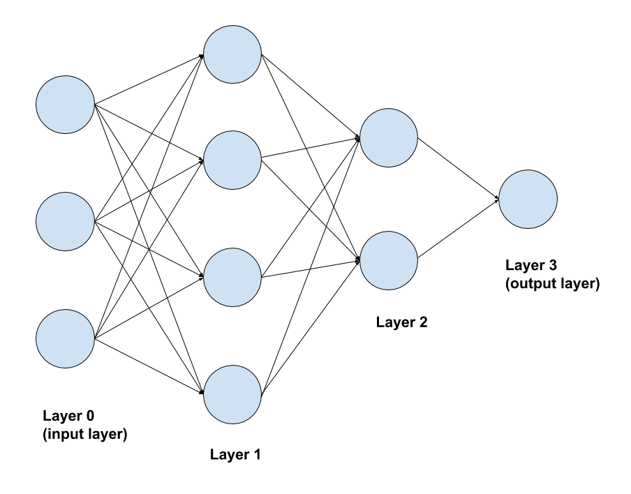
A neural network is a collection of connected neurons, where the output of each neuron is either an input to another neuron or a final output of the network. As a reminder, each neuron has some parameters that describe how to linearly transform its inputs and an activation function. The most basic neural network is the feed-forward neural network, in which the neurons are arranged in sequential layers, where the outputs of neurons from one layer are the inputs to the neurons in the next layer.

The zeroth layer contains the input features (3 features in the picture above) and is usually not counted as a layer when describing a neural network. The above network thus has 3 layers: the first layer has 4 nodes, the second has 2 nodes, and the third (output) layer has 1 node. Working through the depicted example:
- A new observation with 3 features is loaded in the input layer.
- Each node in the first layer takes as input the 3 features in the input layer, applies a linear transformation to these features, and then applies a nonlinear activation function to return a single output. After the output from each node in the first layer is computed, the second layer is evaluated.
- Similar to the first layer, each node in the second layer takes the outputs of the previous layer as input (4 outputs in this example) and returns a single output.
- The single node in the third (and final) layer takes the 2 outputs from the second layer as input and returns one output. For regression and binary classification tasks, the output layer always has 1 node because the network returns one number for each observation.
Layers 1 and 2 are called hidden layers to distinguish them from the output layer. Nodes are sometimes called units and so the nodes in the hidden layers are called hidden units.
The neuron view above is complicated and obfuscates the bigger picture. For more complicated networks, we often draw a layer view.

The layer view emphasizes how many nodes are in each layer (its size) and some other information, such as which activation function is used for all nodes in the layer.
Decision boundaries
The primary task in supervised machine learning is given a set of points \((x_i, y_i)\), ‘‘learn’’ a function \(f\) such that \(y_i \approx f(x_i)\). Neural networks provide a very rich class of functions from which to learn \(f\).
To understand the kind of data we can fit with a neural network, recall that a single neuron can linearly separate data. Suppose we have three neurons (with tanh activations) in the first layer of a neural network, each dividing the two-dimensional feature plane in a different way. Let \(a_1\), \(a_2\), and \(a_3\) be outputs of these neurons and let \(a = a_1 + a_2 + a_3\) be the sum (computed by a neuron in the second layer). The figure below depicts three lines corresponding to decision boundaries of the neurons in the first layer. The shaded regions correspond to different values of \(a\), the output of the second layer.

Notice that \(a = 3\) on the dark blue triangle in the center, but is 2 or less in all other regions. We can thus test if a point belongs to the center triangle by checking whether \(a \geq 2.5\). We just showed how a two-layer neural network can learn a triangular decision region. Similar arguments show that neural networks can capture intersections and unions of half spaces, which allows them to model arbitrarily complex decision boundaries.
In fact, shallow two-layer neural networks can model bounded continuous functions arbitrarily well. Deep learning is crucial, though, because shallow networks do not necessarily model complex functions efficiently. Indeed, there are functions that require exponentially more nodes to model with a shallow network than with a deep network. A more intuitive explanation for why deep learning works better in practice is that the layers in a deep network gradually learn more and more complex structure. For example, the first layer in an image recognition model might learn to recognize edges, the next layer might learn to recognize basic shapes, and so forth.
Composition view
A feed forward neural network is just a composition of a lot of functions. Indeed, the final output of the network is a composition of \(L\) layer transformations
\[a^{[L]}(a^{[L-1]}(a^{[L-2]}(...a^{[2]}(a^{[1]}(x))))),\]where the transformation in the \(l\)th layer \(a^{[l]}(\cdot) = g^{[l]}(l^{[l]}(\cdot))\) consists of a linear function \(l^{[l]}(x) = W^{[l]} x + b^{[l]}\) followed by a nonlinear activation \(g^{[l]}\).
To evaluate the network at a point \(x\), we work from the inside outwards in the composition, first computing \(a^{[1]} = a^{[1]}(x)\), then using \(a^{[1]}\) to compute \(a^{[2]} = a^{[2]}(a^{[1]})\), and so forth. In the layer diagram, this corresponds to going through the network from left to right and is called forward propagation.
The coefficients \(W\) and \(b\) in the linear functions are the parameters of the network. A neural network is usually fit with mini-batch gradient descent or some other first order optimization scheme. This requires computing the derivative of some loss \(\ell\) with respect to the network’s parameters.
The loss is also a large composition
\[\ell \circ a^{[L]} \circ a^{[L-1]} \circ \cdots \circ a^{[1]}.\]Assuming each layer has one node for simplicity, the chain rule gives the following:
\[\begin{aligned} \frac{d \ell}{d a^{[l]}} &= \frac{d \ell}{d a^{[L]}} \frac{d a^{[L]}}{d a^{[L-1]}} \cdots \frac{d a^{[l+2]}}{d a^{[l+1]}} \frac{d a^{[l+1]}}{d a^{[l]}} \\ \frac{d \ell}{d W^{[l]}} &= \frac{d \ell}{d a^{[l]}} \frac{d a^{[l]}}{d W^{[l]}} \\ \frac{d \ell}{d b^{[l]}} &= \frac{d \ell}{d a^{[l]}} \frac{d a^{[l]}}{d b^{[l]}}. \end{aligned}\]To compute the loss derivative with respect to the \(l\)th layer’s parameters, we work from right to left in the network, first computing \(\frac{d \ell}{d a^{[L]}}\), then computing \(\frac{da^{[l]}}{da^{[L-1]}}\), and so on. This is called back propagation.
To summarize
- A neural network is a composition of many functions
- Forward propagation is a graphical way of evaluating the composition
- Back propagation is a graphical way of applying the chain rule to evaluate the derivative of the composition
I will discuss forward and back propagation in more detail in the next post, where I’ll walk through implementing a deep neural network.
Written on August 11th, 2019 by Scott Roy